Data Consolidation In Excel - Part 1

Note: We are not going to discuss here the Consolidation function of Excel. The said function is used if you want to sum up multiple numbers from different Excel files that have same format into a single Excel file. I've got limited time to post to discuss it but will try to tackle it in the near future.

In this post, we will combine records from different files with different format. Appending them all in a single Excel file. No summation will be done.


Data Consolidation

Is it to much tedious if you copy and paste manually sets of data from multiple files and append them all together in a master file? Let's say you have 50 files of records and you open them one by one and copy the records and paste into a single file. And the most boring of all about it is that you need to do it over and over again in a weekly basis. Of course, you will agree with me that it is tedious.

If you find yourself in that situation and don't want to do the same thing manually weekly, then you can automate the whole process. The long hours of doing it manually can be reduced in an hour or two with a macro program.


Source Data

So let's start by creating the files to be combined together. For our example, we will create 3 different source files; an Excel file, CSV file, and a Tab delimited file.

Excel File -- Create a new Excel file and copy the data in the following screen shot and save as Excel file, of course :)














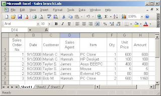
CSV File -- In Excel, copy the data in the following screen shot and save it in CSV format by clicking "Save As" in the File menu. Change the file type to CSV before clicking the Save button.












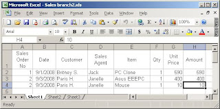
Tab Delimited -- In Excel, copy the data in the following screen shot and save it in Tab delimited text file by clicking the "Save As" in the File menu. Change the file type to "Tab delimited" before clicking the Save button.












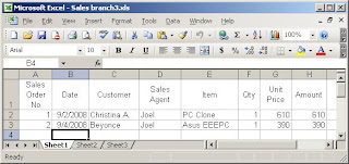
Recording Data Import

AT this point, we will extract records from the files that we created while we are macro recording it. To start the Macro Recorder, please see my post on how to do that at Easiest Way to Learn Excel VBA Programming by Macro Recorder. Once it is up and running, we will do the data extraction of the 3 files. But it is much better if you will start and stop the macro recorder for each file extraction so that each file will have its own procedure module. then we will examine each module one by one to learn the difference.

To extract the file, follow the instruction in my previous post, Export To Excel.

You should generate the same codes as below:

Source Code for Excel file.

Sub Macro1()
    '
    ' Macro1 Macro
    ' Macro recorded 9/14/2008 by Joel.Protusada
    '
    
    '
    With ActiveSheet.QueryTables.Add(Connection:=Array( _
        "OLEDB;Provider=Microsoft.Jet.OLEDB.4.0;" & _
        "Password="""";User ID=Admin;Data Source=" & _
        "E:\Consolidation\Sales branch1.xls;" & _
        "Mode=Share Deny Write;", _
        "Extended Properties=""HDR=YES;"";Jet OLEDB:" & _
        "System database="""";" & _
        "Jet OLEDB:Registry Path="""";Jet OLEDB:" & _
        "Database Password="""";Jet OLEDB:", _
        "Engine Type=35;Jet OLEDB:Database " & _
        "Locking Mode=0;Jet OLEDB:" & _
        "Global Partial Bulk Ops=2;Jet OLEDB:Global " & _
        "Bulk Transactions=1;Jet OL", _
        "EDB:New Database Password="""";Jet OLEDB:" & _
        "Create System Database=" & _
        "False;Jet OLEDB:Encrypt Database=False;Jet " & _
        "OLEDB:Don't Copy Locale", _
        " on Compact=False;Jet OLEDB:Compact " & _
        "Without Replica " & _
        "Repair=False;Jet OLEDB:SFP=False" _
        ), Destination:=Range("A1"))
        .CommandType = xlCmdTable
        .CommandText = Array("Sheet1$")
        .Name = "Sales branch1"
        .FieldNames = True
        .RowNumbers = False
        .FillAdjacentFormulas = False
        .PreserveFormatting = True
        .RefreshOnFileOpen = False
        .BackgroundQuery = True
        .RefreshStyle = xlInsertDeleteCells
        .SavePassword = False
        .SaveData = True
        .AdjustColumnWidth = True
        .RefreshPeriod = 0
        .PreserveColumnInfo = True
        .SourceDataFile = _
        "E:\Consolidation\Sales branch1.xls"
        .Refresh BackgroundQuery:=False
    End With
End Sub

Source code for CSV file.

Sub Macro2()
    '
    ' Macro2 Macro
    ' Macro recorded 9/14/2008 by Joel.Protusada
    '
  
    '
    With ActiveSheet.QueryTables.Add(Connection:= _
        "TEXT;E:\Consolidation\Sales branch2.csv", _
        Destination:=Range("A1"))
        .Name = "Sales branch2"
        .FieldNames = True
        .RowNumbers = False
        .FillAdjacentFormulas = False
        .PreserveFormatting = True
        .RefreshOnFileOpen = False
        .RefreshStyle = xlInsertDeleteCells
        .SavePassword = False
        .SaveData = True
        .AdjustColumnWidth = True
        .RefreshPeriod = 0
        .TextFilePromptOnRefresh = False
        .TextFilePlatform = 437
        .TextFileStartRow = 1
        .TextFileParseType = xlDelimited
        .TextFileTextQualifier = xlTextQualifierDoubleQuote
        .TextFileConsecutiveDelimiter = False
        .TextFileTabDelimiter = False
        .TextFileSemicolonDelimiter = False
        .TextFileCommaDelimiter = True
        .TextFileSpaceDelimiter = False
        .TextFileColumnDataTypes = Array(1, 1, 1, 1, 1, 1, 1, 1)
        .TextFileTrailingMinusNumbers = True
        .Refresh BackgroundQuery:=False
    End With
    Sheets("Sheet3").Select
End Sub

Source code for the tab delimited file.

Sub Macro3()
    '
    ' Macro3 Macro
    ' Macro recorded 9/14/2008 by JPCORP
    '
  
    '
    With ActiveSheet.QueryTables.Add(Connection:= _
        "TEXT;E:\Consolidation\Sales branch3.txt", _
        Destination:=Range("A1"))
        .Name = "Sales branch3"
        .FieldNames = True
        .RowNumbers = False
        .FillAdjacentFormulas = False
        .PreserveFormatting = True
        .RefreshOnFileOpen = False
        .RefreshStyle = xlInsertDeleteCells
        .SavePassword = False
        .SaveData = True
        .AdjustColumnWidth = True
        .RefreshPeriod = 0
        .TextFilePromptOnRefresh = False
        .TextFilePlatform = 437
        .TextFileStartRow = 1
        .TextFileParseType = xlDelimited
        .TextFileTextQualifier = xlTextQualifierDoubleQuote
        .TextFileConsecutiveDelimiter = False
        .TextFileTabDelimiter = True
        .TextFileSemicolonDelimiter = False
        .TextFileCommaDelimiter = False
        .TextFileSpaceDelimiter = False
        .TextFileColumnDataTypes = Array(1, 1, 1, 1, 1, 1, 1, 1)
        .TextFileTrailingMinusNumbers = True
        .Refresh BackgroundQuery:=False
    End With
End Sub

As you can see there are almost no difference between the CSV and Tab file. So in our programming we will modify the codes above and we will create a single subroutine to handle both CSV and Tab files, and a separate subroutine for Excel files.


Project Details

Before we start with the actual programming, we need to be precised in the parameters of our consolidation. Below is the brief specifications of it:

• To trigger the consolidation, an option in the menu should be added to run it. To do that visit my post Create Customize Excel Menu.
  
• All the files to be consolidated should be residing in the same folder as the master file. The master file is an Excel file that will serve as the repository of all the records. It also has the consolidation macro program.
• There will be only three data file formats to be recognized by the program; Excel, CSV, and tab delimited. If there is a need for other format, you can easily modify the program that we will make here.
• program should follow the flow chart below:

Modified Macro Program

As I've said we will modify the code above to subroutines that we can use and reuse in our programming. Below is the modified recorded macro for the Excel file extraction:

Sub ExtractExcelData(strPath As String, _
strFile As String, strSheet As String)
Sheets(strSheet).Select
With ActiveSheet.QueryTables.Add(Connection:=Array( _
 "OLEDB;Provider=Microsoft.Jet.OLEDB.4.0;" & _
 "Password="""";User ID=Admin;Data Source=" & _
 strPath & strFile & ";Mode=Share Deny Write;", _
 "Extended Properties=""HDR=YES;"";Jet OLEDB" & _
 ":System database="""";Jet OLEDB:Registry Path="""";Jet OLEDB" & _
 ":Database Password="""";Jet OLEDB:", _
 "Engine Type=35;Jet OLEDB:Database Locking Mode=0;" & _
 "Jet OLEDB:Global Partial Bulk Ops=2;" & _
 "Jet OLEDB:Global Bulk Transactions=1;Jet OL", _
 "EDB:New Database Password="""";Jet OLEDB:" & _
 "Create System Database=False;Jet OLEDB:" & _
 "Encrypt Database=False;Jet OLEDB:Don't Copy Locale", _
 " on Compact=False;Jet OLEDB:Compact Without Replica " & _
 "Repair=False;Jet OLEDB:SFP=False" _
 ), Destination:=Range("A1"))
 .CommandType = xlCmdTable
 .CommandText = Array("Sheet1$")
 .Name = "Sales branch1"
 .FieldNames = True
 .RowNumbers = False
 .FillAdjacentFormulas = False
 .PreserveFormatting = True
 .RefreshOnFileOpen = False
 .BackgroundQuery = True
 .RefreshStyle = xlInsertDeleteCells
 .SavePassword = False
 .SaveData = True
 .AdjustColumnWidth = True
 .RefreshPeriod = 0
 .PreserveColumnInfo = True
 .SourceDataFile = strPath & strFile
 .Refresh BackgroundQuery:=False
End With
End Sub

To test the above procedure, the correct parameters should be supplied like the example below:

Sub TestExtractExcelData()
ExtractExcelData "E:\consolidation\", "Sales branch1.xls", "sheet4"
'Parameters are:
'strPath - folder where to get the file
    'strFile - Excel filename of the source data.
    'strSheet - woeksheet where to put the data.
End Sub

Here's the subroutine for the CSV and Tab files extraction:

Sub ExtractTextData(strPath As String, _
strFile As String, strSheet As String, isCSV As Boolean)
Dim MyRecords
Sheets(strSheet).Select
If isCSV Then
   Set MyRecords = ActiveSheet.QueryTables.Add(Connection:= _
   "TEXT;" & strPath & strFile, Destination:=Range("A1"))
Else
   Set MyRecords = ActiveSheet.QueryTables.Add(Connection:= _
   "TEXT;" & strPath & strFile, Destination:=Range("A1"))
End If
With MyRecords
   .Name = Left(strFile, Len(strFile) - 4)
   If isCSV Then
       .TextFileCommaDelimiter = True
       .TextFileTabDelimiter = False
   Else
       .TextFileCommaDelimiter = False
       .TextFileTabDelimiter = True
   End If
   .FieldNames = True
   .RowNumbers = False
   .FillAdjacentFormulas = False
   .PreserveFormatting = True
   .RefreshOnFileOpen = False
   .RefreshStyle = xlInsertDeleteCells
   .SavePassword = False
   .SaveData = True
   .AdjustColumnWidth = True
   .RefreshPeriod = 0
   .TextFilePromptOnRefresh = False
   .TextFilePlatform = 437
   .TextFileStartRow = 1
   .TextFileParseType = xlDelimited
   .TextFileTextQualifier = xlTextQualifierDoubleQuote
   .TextFileConsecutiveDelimiter = False
   .TextFileSemicolonDelimiter = False
   .TextFileSpaceDelimiter = False
   .TextFileColumnDataTypes = Array(1, 1, 1, 1, 1, 1, 1, 1)
   .TextFileTrailingMinusNumbers = True
   .Refresh BackgroundQuery:=False
End With
End Sub

Here's the code to test it.

Sub TestExtractCSVData()
ExtractTextData "E:\consolidation\", _
"Sales branch2.csv", "sheet5", True
End Sub

Sub TestExtractTabData()
ExtractTextData "E:\consolidation\", "Sales branch3.txt", _
"sheet6", False
End Sub
'Parameters are the same as in the Excel routine.
'The fourth parameter is a boolean type which
'means that if the TRUE, it is a CSV file,
'otherwise Tab file. 

So there you go. Those are the codes to do it. I will post soon the whole VBA program as it is too long to include it here.

Click here to subscribe and receive Pro-business Excel VBA Programming tips.

If you like this post in Pro-business Excel VBA Programming, buy me a coffee.

Export To Excel

This is the first part of our discussion on how to export data to Excel. We will start with the simplest one; how to transfer data from a flat file (CSV, Tab delimited, PSV, etc.) to Excel. Let's know first what is a flat file...


What is a flat file?

Wikipedia described it best...

A flat file is a file that contains records, and in which each record is specified in a single line. Fields from each record may simply have a fixed width with padding, or may be delimited by whitespace, tabs, commas (CSV) or other characters. Extra formatting may be needed to avoid delimiter collision. There are no structural relationships. The data are "flat" as in a sheet of paper, in contrast to more complex models such as a relational database.

In short it's an ordinary file that stores records in sequential order.

This simple pattern of records saved in a file makes it possible for Excel to extract them and load into worksheet cells. A function is available in Excel to do it with a wizard tool.


Export To Excel

1.) Before we can export records to Excel, we need to have source file. So, let's create one by opening Windows Notepad and enter the set of data exactly as shown in the screen grab below:













The sample records I created are list of customers. Each field should be separated by a Pipe ("|") character. After entering the string above, save the file. In my case, I named it Customer. The filename would have a .TXT extension, but since our data is pipe delimited, we should rename the extension to .PSV (Pipe Separated Value). We have now Customer.PSV.

2.) Create a new Excel worksheet. On the menu, click Data>Import External Data>Import Data as shown below:




















3.) This will bring out the Select Data Source window:














In this window, you will see many choices in the "Files of type" pull down list but you need only to choose All files (*.*) because PSV format is not included in the list. Locate the Customer.PSV then double click it.

4.) The Text Import Wizard appears as shown below. Do not change the default Delimited in the Original data type as our records are delimited by a pipe character. Click Next button.
















5.) The second screen of the wizard appears. Check the Other check box and put a pipe in the text field next to it. See below how. Then click Next button.
















6.) The third screen of the wizard appears (see below). Here you usually indicate the data type of each column. But in the case of our sample records, we will just click Finish button.
















7.) The Import Data window pops out, choose Existing worksheet since we juist created a new one and click Ok to store all the records in the worksheet as shown in the screen grab below:















We are done.

Now you know how to export records from a text file into Excel and having these records in the worksheet you can now manipulate the data the way you want. You can pivot them to summarize and come up with useful information, or you can consolidate them with other data extracted from other source, etc.

In my next post, we will discuss consolidation of records from different files using VBA programming.

Happy Weekend :)

Click here to subscribe and receive Pro-business Excel VBA Programming tips.

If you like this post in Pro-business Excel VBA Programming, buy me a coffee.

Pareto Chart Example

I will give you a very simple Pareto chart example. Create a new workbook and enter exactly the same figures in the screen shot below:





















The worksheet above is an example of list of reasons why you lost business proposals or quotes to other competitors. Column A has the reason descriptions. Column B has the corresponding number of times with that lost reasons in Column A. Column C has the percentages. Column D is the running percentages of Column C.

Highlight the range A1 to A6. Press Ctrl key simultaneously on highlighting the C1 to D6. Then click the Insert>Chart in the menu. The chart wizard will appear on the screen for you to choose the kind of chart that you want to create. Choose the Bar Chart. Click the finish button to display the chart equivalent of the table you selected. Right-click once one of the Running % bar and choose Chart Type in the menu that appears. The Chart Type window will pop out and then you can change Running % from bar to line type. The chart should look like the screen shot below:






















Now you know how to create your own Pareto chart, but you probably have questions at the back of your head right now. And you might be asking the following questions:

1. I can't see the 80% and 20% in the chart so why is it called 80-20 rule based?
2. How this chart can help the business?
3. How this chart can be applied with a database with large repository of data?

I will try to answer these questions the best that I can.

1. ) I can't see the 80% and 20% in the chart so why is it called 80-20 rule based?

Answer: I intentionally made the sample Pareto chart an imperfect one to make it looks like a realistic one. The 80-20 rule doesn't mean that exactly 20% of the reasons are 80% of the root causes of losing businesses. It simply states the principle that a few of the reasons causes the majority of why you are losing, not exactly 20%. That's why the phrase "the vital few and the trivial many" was coined after this rule.

2.) How this chart can help the business?

Answer: Considering the example above, you can easily see that most of the reasons in losing a business are Price and Customers' Lack of Fund. The two reasons when combine together have more than 50% and simply means they are major root causes of your loses. Knowing that information, you can focus in those problem areas; you can act and fix on those situations. Once the problems are solved in those areas, you also solved more than 50% of the root causes and surely will improve your business performance and profitability. Then you can generate again another Pareto chart to know if the situation has changed and then focus again in the majority root causes. It is a continuous cycle of knowing the big problems and solving them.

3. How this chart can be applied with a database with large repository of data?

Answer: This is the most important part of our discussion. In your company, you surely have a lot of records sitting in your Excel files, Access files, SQL Server, Oracle, etc. How can we use them to create a Pareto chart.

Our example above is very simple that you don't need to convert it to Pareto chart to know what are the majority of the problems. But imagine, for example, if you have many branches, let's say 30 branches with 10 sales persons each that have multiple prospective customers and they are recording those leads pipeline in Excel to monitor quote status, amount, products, etc. Do you think you can easily come up with a Pareto chart with many Excel files in different locations? No, it's not that easy to consolidate those data. You need to have a procedure in implementing the consolidation and a good Excel macro program to automate the stitching of the records.

Another good example is: you are in a manufacturing company and having an ERP system. You want to create a Pareto chart because you want to know from which of the 60,000 raw materials that take most of your inventory investments. It is because you want to focus on them to make sure that majority of your investment is taken care of by keeping an eye on the correct reorder point, correct stock handling, good supplier selection, proper purchasing approval, etc. And with it, you can delegate the "trivial many" to your subordinates.

In my subsequent posts, I will demonstrate to you a different methods of how to export to excel records from different platforms (mostly with VBA programming); flat file, Excel, Access, SQL Server (OLAP or not) and Oracle. It will be a series of posts as I can not tackle them all in a sigle posting.

Subscribe now. You can see below how.

Click here to subscribe and receive Pro-business Excel VBA Programming tips.

If you like this post in Pro-business Excel VBA Programming, buy me a coffee.

Pareto Chart

The Pareto Chart, also known as the Pareto Analysis, ABC Analysis, or 80-20 Analysis, is based on the principle of "the vital few and trivial many" developed by Vilfredo Pareto, an Italian economist born in 1848. I'm not going to discuss here his life; you can already research on that in Wikipedia or Google. What you will read here is about the importance of his statistical findings, the 80-20 rule, that you can apply in almost every aspect of your life, especially in business. And in business, I will give you an example in my next post on how can you make the Pareto chart as a decision support tool by digging and using the data that you already have in your existing database. Yes, the raw data residing in your database, whether it's an Excel data, MS Access data, OLAP data, SAP data, or Oracle data, are just sitting there waiting to be dug up and be transformed to an information that will greatly help you to improve your business focus, operation, and eventually profitability.

The 80-20 rule means that approximately 20% of everything is either better or worse than the 80%. For example, 20% of your retail products are making 80% of your profitability. 20% of your sales agents are giving the 80% of the total sales. And here's a more enlightening; in an equally managed inventory of raw materials, 80% of your inventory investment goes to a certain small group of products that need more attention than the 20% that you can delegate to someone else. There are actually limitless applications to this theory. All you have to do is think outside the box and hard.

In the next post, the example I promised you will be discussed and in the subsequent posts thereafter, the different way to extract data from different sources (Flat file, Access, SQL Server, SAP and Oracle E-Business Suite) will be discussed. So be in the loop. Subscribe now. You'll see below how.

Click here to subscribe and receive Pro-business Excel VBA Programming tips.

If you like this post in Pro-business Excel VBA Programming, buy me a coffee.

Excel Data Entry Form

Here is a simple way to make your Excel worksheet as a simple database. In our example, we will create a vendors table and we will use an Excel data entry form to allow user to populate the vendors table. Here's how to do it...

Step 1: Create a new workbook. Rename the first worksheet as "Vendor". It will become the repository of the vendor information that the users will enter to our data entry form.

Step 2: At the first row, enter the following "column" names...

• Vendor ID
• Vendor Name
• Address 1
• Address 2
• City
• Country
• Zip
• Phone 1
• Phone 2
• Fax
• Contact

Here's how the worksheet should look when you enter them:


These "column" names are just example of what you can put in a vendor table. You can add your own columns or delete some that you think you don't need in your own application.

Step 3: Select all the cells of the column names.

Step 4: At the menu, click Data>Form as seen in the screen shot below:

You will be prompted with multiple questions; but your answer should be to make the first row of the highlighted cells as the columns (or labels). This question is only when the excel database has no records in it. The next time, when there are already records in it, this will not appear. The "Ok" button should be pressed at this point.

Step 5: The Excel data entry form is now in front of you. Here's how it looks...


Step 6: Like a usual data entry form, there are things that you can do with the form. To enter a new record, enter the information in each field and click the "New" button. "Delete" button is used to delete a record. "Restore" button is used to restore previous content of the fields when you amend the fields. "Find Prev", "Find Next" and "Criteria" are for records navigation. I have to say that most of the time the "Criteria" is not functioning well or maybe I was doing something wrong to make it act unusual.

So that's how to go through the Excel data entry form. This small database management is should be enough for small needs, but as the needs grow new methods are should be used instead of this. In the upcoming posts in the near future, I will discuss other ways to do that. not all in a single post, but in a subsequent series of posts.

You better subscribe now. See below how...

Click here to subscribe and receive Pro-business Excel VBA Programming tips.

If you like this post in Pro-business Excel VBA Programming, buy me a coffee.

Checking Excel's Filename

This is an improvement of my previous post. It always happens to me that whenever I put a password protection in my Excel/VBA program, I need to hide to the regular users not just the confidential data or customized menu, but the password window also should not displayed so that they will not have the idea that the file has a confidential information or has features that they shouldn't see.

This is a simple trick that I've been using for years. Open the program that we did in the last post and change code in Open event in the ThisWorkbook object as indicated below:

'this is the original code

Private Sub Workbook_Open()
PasswordOk = False
frmPassword.Show
End Sub


'change it to this one

Private Sub Workbook_Open()
PasswordOk = False
If Left(ThisWorkbook.Name, 5) = "SYSAD" Then
   frmPassword.Show
End If
End Sub

As you can see the program simply checks the filename of the Excel file if it is prefixed by the word "SYSAD". If it is, it will prompt for the password, otherwise, it loads just like an ordinary Excel file.

To ordinary users of the file you can just send to them a copy of the file without the prefix "SYSAD". To all users that needs to have access to the protected worksheet and customized menu, you can send to them the file with "SYSAD".

Click here to subscribe and receive Pro-business Excel VBA Programming tips.

If you like this post in Pro-business Excel VBA Programming, buy me a coffee.

Excel Password Protection - Part 4

There are situations that you need to hide a customized menu or to make worksheets read only from certain users that need your Excel file for informational purposes only and they shouldn't mess around with the important or confidential data in the worksheets.

This is the final post of the 4-part article about Excel Password Protection. We'll discuss here how to create a VBA program to make your worksheets and customized menu safe from unauthorized users. Just follow the steps below:

Step 1: From the previous post, open the file that we created. It should have the menu program that we entered in it. Open the VBE (you should know it by now or read the previous post, click here to learn about it).

Step 2: Create a new user form by clicking Insert>UserForm. The user looks like the screen shot below. It's the UserForm1. Beside it you'll see the Toolbox menu. It is used to put controls inside the form like a button, label and a text field.

Step 3: Open up the properties window by clicking View>Properties Window or by pushing F4 key. The properties window looks like the figure below:

Step 4: Click the new user form so that the properties window will show the form's properties. Inside that properties window, change the following form properties:

• Name: change it to "frmPassword"
  
• Caption: change it to "Enter Password"
  
• Height: 111
  
• Width: 210

Step 5: From the tool box window, drag and drop one label, textbox and a button to the user form. Once controls are put in the form, change the properties of each according to the values below:

Label

• Name: lblPassword
  
• Caption: Password
  
• Width: 42
  
• Height: 12
  
• Top: 28
  
• Left: 24
  

Textbox

• Name: txtPassword
  
• Width: 120
  
• Height: 18
  
• Top: 24
  
• Left: 72
  

Button

• Name: cmdOk
  
• Caption: Ok
  
• Width: 48
  
• Height: 18
  
• Top: 60
  
• Left: 144

Step 6: Create a new module by clicking Insert>Module in the VBE menu. At the new module enter the following code: (copy-paste will do it quick)

'indicator that password is ok or not
'true = ok, false is not
Public PasswordOk As Boolean

'temporary storage of the
'password entered by the user
Public strPassword As String

Sub UnlockSystem(strPW As String)
 PasswordOk = False 'initialize to false

  'if password entered is incorrect
  'it will generate an error and
  'will not proceed in menu activation
 On Error GoTo MyErr
    Sheet1.Unprotect Password:=strPW
    PasswordOk = True
    strPassword = strPW
    PutProBusinessMenu
 On Error GoTo 0
 Exit Sub
MyErr:
 MsgBox "Worksheet 1 will remain locked and" & _
 " customized menu is hidden.", , "Invalid Password"
End Sub

Sub LockSystem()
 'this will be used to lock the program
 'and disable the customized menu
 'when changing workbook and closing the file
 If PasswordOk Then
    Sheet1.Protect Password:=strPassword
    ClearProBusinessMenu
 End If
End Sub

Step 7: Go back to the user form and double click the button control in it. The code view for the button is displayed. Enter the following code inside it:

'when the ok button is clicked,
'it runs the UnlockSystem routine
Private Sub cmdOk_Click()
 UnlockSystem txtPassword.Text
 Unload Me
End Sub

Step 8: Finally change the code of the entire ThisWorkbook object and put the following code:

Private Sub Workbook_Activate()
  'if a workbook is activated,
  'it will unlock the system if password
 'previously entered was correct
 If PasswordOk Then
    UnlockSystem strPassword
 End If
End Sub

Private Sub Workbook_BeforeClose(Cancel As Boolean)
  ;lock again the system before closing
 LockSystem
End Sub

Private Sub Workbook_Deactivate()
  'locking the system when workbook is deactivated.
 LockSystem
End Sub

Private Sub Workbook_Open()
  'when the file is open, it prompts for the
  'password
 PasswordOk = False
 frmPassword.Show
End Sub

Step 9: Lastly, lock the first sheet of your excel file (the one that has the object name of Sheet1) using any password that you want. The same password will be used to unlock it and enable the menu.

There you go. try to run the program by closing the file and reopen it. The file will ask for the password. If the correct password is entered, you will see the customized menu and the worksheet is unlocked. Otherwise, menu and worksheet is locked.

Click here to subscribe and receive Pro-business Excel VBA Programming tips.

If you like this post in Pro-business Excel VBA Programming, buy me a coffee.

Create Customize Excel Menu

I have to apologize that I put off the supposedly next password article for this one. I must discuss this one first because the next password article will need this program module routines. I will be discussing here how to create a customize menu that we can insert in the existing Excel menu. The menu can be used in your program applications in many ways so it is something that you should know when developing Excel programs.

So let's get started to create our own customized menu.

Step 1: Open you Excel file and run the Visual Basic Editor (VBE) by clicking Tools>Macro>Visual Basic Editor.

Step 2: When VBE appears, add a new module by clicking Insert>Module at the VBE menu.

Step 3: At the new module, enter the following code snippets:

Sub PutProBusinessMenu()
    Dim cmdControl As CommandBarControl
    Dim cmdbarMenu As CommandBar
    Dim cmdControlMenu As CommandBarControl
    Dim intHelpMenuItem As Integer

    ClearProBusinessMenu

    Set cmdbarMenu = _
    Application.CommandBars("Worksheet Menu Bar")
     
    intHelpMenuItem = _
    cmdbarMenu.Controls("Help").Index
     
    Set cmdControlMenu = _
    cmdbarMenu.Controls.Add(Type:=msoControlPopup, _
    Before:=intHelpMenuItem)
                  
    cmdControlMenu.Caption = "&Pro-business"
     
    With cmdControlMenu.Controls.Add( _
    Type:=msoControlButton)
        .Caption = "Execute Process"
        .OnAction = "ExecuteProcess"
    End With
End Sub

Sub ClearProBusinessMenu()
    On Error Resume Next
    Application.CommandBars("Worksheet Menu Bar"). _
    Controls("&Pro-business").Delete
    On Error GoTo 0
End Sub

Sub ExecuteProcess()
    MsgBox "Process is executed."
End Sub

The first snippet is about creating the menu before the Help option. The second one is deleting it from the menu. You need the second snippet to clear your own menu when the file is closed or when the user move from your workbook to another workbook that doesn't use your program. The next step is about doing that.

The last snippet is the module to be executed when the option in our new menu is executed. This part is where you put your own code when you want to use this program in your own application.

Step 4: Click ThisWorkbook item in the Project window at the left side of your VBE. When the ThisWorkbook module opens up and enter the following code snippets.

Private Sub Workbook_Activate()
    PutProBusinessMenu
End Sub

Private Sub Workbook_Deactivate()
    ClearProBusinessMenu
End Sub

Step 5: Save your Excel file, close it and try to open it again. You will see that you have the new menu right before the Help in the main menu. Open up another Excel file and try to switch between our Excel file and the other one. You will see that the menu appears only when our Excel file is active.

That's how to do it. Next time, as promised, the Excel password protection for your Excel and VBA program. We will put a password protection to this customized menu and we will discuss so much more about Excel program security.

Subscribe now to see the next topic by clicking the link below:

Click here to subscribe and receive Pro-business Excel VBA Programming tips.

If you like this post in Pro-business Excel VBA Programming, buy me a coffee.

Excel Password Protection - Part 3

In our 2 previous posts, Excel Password Protection Part 1 & Part 2, we tackled 2 ways to protect your Excel spreadsheets. The first part was about protecting the Excel file itself. The second was about security at the worksheet level.

We are now in the third part of Excel Password Protection series. It's time discuss how to give security to your valued source code. Here are the steps:

1.) Open your Excel file with the VBA program. Load the VBE from the menu by clicking Tools>Macro>Visual Basic Editor.

2.) At the VBE menu, click Tools>VBAProject Properties and the Protection tab. Its window look like the screen shot below:

3.) Tick the checkbox to lock the project's code for viewing and at the last part of the window, you need to enter your password in both the "Password" and "Confirm Password" text fields. This is to make sure that you didn't put in a misspelled one.

4.) Click OK button

So that's it. Isn't it simple. The next time you open your Excel file and its VBE, you will not see your program unless you enter the right password.

In this Part 1-3 of Excel Password Protection series, we haven't done any programming yet, but in the next post, you will learn how to make your own VBA program to protect some portion of your Excel file from unauthorized access, execution or modification. You haven't seen the best part yet. So you better come back here. Subcribe now for free by clicking here.

After this password series, I will start to discuss (mostly) about business processes and Excel and VBA can be a good part of them. Right now, I've been thinking what to tackle first. I want you, my readers, to help me out on what particular interest most of my readers are into. I want to give what you want, so please help me by voting at the "Poll" section at the right side of this page. The one that has the highest vote will be touched here first.

Start voting! :)

Click here to subscribe and receive Pro-business Excel VBA Programming tips.

If you like this post in Pro-business Excel VBA Programming, buy me a coffee.

Excel Password Protection - Part 2

In this second post about Excel Password Protection, we will discuss how to protect individual worksheet of an Excel workbook. There are many reasons why sometimes we need to password protect them but most of them are for keeping the content of the worksheet intact and unmodified, or keeping the confidentiality of the content, e.g. formula for profit margin, item cost, etc. from those who shouldn't be looking at them. Without so much bother, here are the ways to password protect your worksheets.


Making A Worksheet Read-Only

To protect your worksheet from alteration and to hide all the formula in all the cells by locking them by a password, all you have to do is choose the tab name of the worksheet. Highlight the whole worksheet by clicking the upper left cell header. Then on the menu click Format>Cells. The Format Cells window will appear. Click the Protection tab. It looks like the screen grab below:


There are two checkboxes, the Locked and Hidden checkboxes. The Locked is checked by default but the other one is not. The Locked is to make all the cells unmodifiable when you activate the worksheet password protection. The Hidden checkbox is to hide all the formulas of the cells. Check them both.

The next step is to activate the sheet protection. Go to Tools>Protection>Protect Sheet. You will see the Protect Sheet window as seen below:


The first checkbox you see should be checked to make the security active. The textbox below it is for the password. It is actually optional but what's the use of locked sheet without a password. Anyone can undo the protection when there's no password. So, you should put your password for total guarantee that it's safe.

Below the textbox, you can see a set of checkboxes. Most of the time, I didn't change the default value of them but there's no harm in exploring it. You can experiment on different combinations that you think appropriate to your needs.

When done, push the Ok button to complete the operation. Your worksheet is now read-only protected.


Making Other Cells Unlocked And Changeable

At the above procedure, you locked all the cells and made them unchangeable. But if you need to leave other cells in the worksheet unlock and available for user to alter them, it is also possible to do that. After locking all the cells, you can choose the cells that you want to be kept changeable and highlight them. Click again the Format>Cells at the menu. Choose the Protection tab. Uncheck the Locked checkbox and click Ok button. Activate the sheet protection.

Maybe you are asking, "Why do I have to do that; leaving other cells changeable?". At this level of discussion, it doesn't look like it make sense. Doesn't it? Allow me to give you an example. Let's say, you are making a data entry for a Purchasing Order form. You create a template of the form in Excel and you want the user or the buyer to use that Excel file to create the PO form for the company purchases. At this scenario, you can lock the sheet for the PO entry form to protect the layout from accidental changes and leaving only those fields for the entry of PO number, vendor, payment terms, delivery date, etc. open for user encoding. Do you get the idea?

There are so many things that you can do with the functions. The example I gave above is just one of them and it's a very simple one. Different applications with this is only a matter of how you use your imagination and creativity. I'm sure, you can think of something that you can do with it in you job or business.

Next post will be about Visual Basic protection. So keep the subscription and stay in the loop. To those who want to subscribe, it's for free. Just click here.

Click here to subscribe and receive Pro-business Excel VBA Programming tips.

If you like this post in Pro-business Excel VBA Programming, buy me a coffee.

Excel Password Protection- Part 1

One of my readers, his name is Stew, requested me to discuss about Excel password protection because I mentioned it in my last post entitled Advantages And Disadvantages Of Microsoft Excel Database Application. As I said in that post, there are many ways to protect your Excel file. I can not tackle everything in one post, so consider this as the first part of series of articles about Excel password protection. I put off for a while my topic on how to develop Excel database application to give way to this one.

Password Protect Your Excel File From Unauthorized Use

This one is very simple to do. Open an Excel file. If you just created an unsaved new one, save it first before you can set a password into it. Then follow the steps below:

• Click File>Save As in the menu.
• On the Save As window, click the Tools at the upper right portion of it as shown in the screen shot below:
• The Save Options window will appear as shown in the figure below. The window prompts for 2 passwords. The password to open the file and another one to allow the user to modify the file. The second one is optional. If it is left blank, Excel assumes that the first password is for both opening and modification. If the second password is provided, it will ask for a second password when you open the file. If the second file is not entered on opening, the file is in read-only mode.
• There are two checkboxes, the "Always create backup" checkbox makes your Excel file to create a backup whenever you modified the file. The next one is "Read-only recommended" checkbox that prompts you if you want to open it as a read-only or not.
• The best part of this Excel password protection is that you can tighten your security even more by having a strong encryption method for your password. You can do that by clicking the "Advanced" button. You will see Encryption Type window and choose the encryption type that you want. It looks like this:
• Click the Save button.

Next time we will discuss about password protecting your worksheets and cells ranges.

Click here to subscribe and receive Pro-business Excel VBA Programming tips.

If you like this post in Pro-business Excel VBA Programming, buy me a coffee.

Advantages And Disadvantages Of Microsoft Excel Database Application

Yes, it is possible to make Excel as a database and be able to be a database application just like Access. I am sure that you won't believe me when I say that anything that you can do with a regular programming language is also possible with Microsoft Excel.

But of course, there are advantages and disadvantages in using Microsoft Excel as database. What are the advantages?

• First and foremost, if you have the Microsoft Office in your PC, you don't need anything else to be installed in your computer. You are good to go and can start with your programming straight away.
• Second, if you are a beginner, you can easily learn the Excel VBA Programming because you are half familiar with the programming platform that you are going to use, which is Excel.
• Third, you can start with small Excel database application and as the need grows especially on records that are getting huge, you can still use the same Excel application and upgrade your database platform from Excel to other high-end databases like Access, SQL Server, Oracle, MySQL, etc.
• Fourth, Excel is capable of connecting directly to OLAP databases and can be integrated in Pivot Tables.
• Fifth, You don't need to create a your own financial modules. Excel is rich in financial functions like Fixed Assets Depreciation, Amortization, etc.
• Sixth, Excel is portable. You can send it to someone through email.
  

Excel database application also has its disadvantages. But these disadvantages are sometimes have some workaround that can be done to fix or sometimes there are little effect that you can just live with them. Here are the disadvantages:

• When you develop your application into one file it can be huge and will make your program execution very slow. But as I told you, there are workarounds. Design your program to have compact codes to lessen the bloating of the file. Another way is to separate each application function into more than one files. For example, if you are going to design a purchasing program, you can separate each of them; the purchase requisition function, item-and-price comparison matrix function, vendor master list maintenance, item master list maintenance, purchase order function, etc. Each will have small file, therefore execution is faster.
• When you separate functions to multiple files, Excel files are prone to get lost in your hard drive especially when you break your application to too many files. You should practice a good folders/sub-directories management.
  
• Excel worksheet as a database has a limited number of rows or records that you can store. But when you reach the 65k lines limit, you can convert it easily to Access and the rest of the application is can still be used.
• If you can send Excel via email, you can accidentally send your file to someone who should not have it or not authorized to have it. Solution? You can password protect your Excel file. You can do it in two ways. First, Excel is capable of password protection in many ways (I will also discuss that in the future). Second, you can create your own password protection by Macro/VBA programming.
  

So far there are only 4 disadvantages that I can think of. Of course, some of you has something to say about an Excel as a database application, either positive or negative. But one thing is for sure, if it is a negative one, there is always a solution and you can always do something to fix it.

In subsequent posts, I will give some examples on how to create Excel database application. Everything can not be touched in one writing so it can be a series of posts that you should follow. To be informed of subsequent posts, subscribe to this blog. It's for free and can be done in a few seconds. Just click any of the subscription method on the upper right part of this webpage or just click here.

Click here to subscribe and receive Pro-business Excel VBA Programming tips.

If you like this post in Pro-business Excel VBA Programming, buy me a coffee.

Resizing Excel Radio Button's Font

Someone asked me today on how to change the size of radio button's font. In this kind of situation, the first thing that comes to mind is to use the font resizing function for the cells. But, you can not use it to a form control like the radio button.

To change the font size of a form control, right click on the radio button and choose "Properties" in the pop-up menu that appears. The properties window will be displayed as shown in the screen shot below:



Click the 3-dot button at the rightmost portion of the "Font" property. The font window will appear and therefore you can change the radio button's font. The font window looks like the following figure:



After choosing the size you desire, click the "Ok" button.

You're done.

Click here to subscribe and receive Pro-business Excel VBA Programming tips.

If you like this post in Pro-business Excel VBA Programming, buy me a coffee.

Cursos De Forex: Automatic Currency Conversion Calculator In Excel

Scenario:

You have a spreadsheet that has amount in US Dollar and you need to convert it to other currency. The conversion should be done automatically whenever the workbook is open. The currency rate should be based on the latest conversion rate. As an example, let's say the conversion would be from US Dollar to Singaporean Dollar. How can we do this?


Solution:

In this situation, we are going to use a web query to capture the current currency rate in the Internet and the "open event" whenever the spreadsheet is open. In this case, we will use the Yahoo Finance Currency Conversion Calculator to provide us the most updated rate that we need.


Here are the step-by-step instructions on how to go about it:

1.) Create a new workbook and rename the first worksheet as "Amount". Rename the second as "Currency Rate".

2.) Open your browser and go to Yahoo Finance Currency Conversion Calculator by clicking this: http://finance.yahoo.com/currency

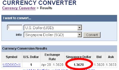
3.) In the "Currency Converter", Put 1 in the TextBox, then choose "US Dollar" in the first dropdown list and Singapore Dollar in the second one as shown in the figure below:



4.) Click the "Convert" button. Yahoo will display the currency conversion rate of the current date as shown below:



5.) Copy the URL: http://finance.yahoo.com/currency/convert?amt=1&from=USD&to=SGD&submit=Convert

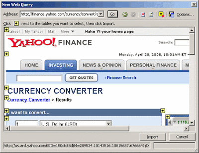
6.) Going back to Excel, click the "Currency Rate" worksheet tab and place Cell A1 as the active cell. In the menu, click Data>Import External Data>New Web Query. The Excel Web Query will appear and in the "Address" field, put (paste) the URL that you just copied and click the "Go" button. See the screen shot below to know how it looks:



7.) Scroll down the window at the portion where you can see the actual conversion rate of USD to SGD. At the left side of it, you will see a small yellow square with an arrow inside pointing to the right. Click on that yellow square and it will change to green color and the arrow will be changed to a check mark as shown in the figure below:



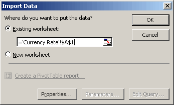
8.) Click the "Import" button. The "Import Data" window will be displayed as shown below and then click the "Ok" button.


9.) The conversion table is now in Excel. Cell E3 has the rate from USD to SGD. Cell C3 has the date of the rate. Click now the "Amount" tab in Excel and put the following in the indicated cells:

• At Cell A1, write "USD Amount"
• At Cell B1, write "SGD Amount"
• At B2, put the following formula "=A2*'Currency Rate'!E3"
• A2 will have the USD Dollar amount to be converted. Initially, let's put 100 dollar in it.
  

10.) Open up the Visual Basic Editor (VBE) and write the following code in "ThisWorkBook" object:

Private Sub Workbook_Open()
    Sheets("Currency Rate").Select
    Selection.QueryTable.Refresh BackgroundQuery:=False
    Sheets("Amount").Select
End Sub

That's all it takes to do it. Whenever you open up the Excel file, it will automatically update the currency rate and eventually the Singapore Dollar amount in Cell B2 in worksheet "Amount".

Now that you know this and by using your imagination, you can play around with it and make something useful out of it. You can apply the technique to your financial or business calculation.

Click here to subscribe and receive Pro-business Excel VBA Programming tips.

If you like this post in Pro-business Excel VBA Programming, buy me a coffee.

TAB Space Adjustment

I am a little bit off topic with this one but if someone in my office is having this kind of problem then most likely some of the million of users of MS Word around the world are also searching for a way to solve it.


Here’s the scenario:

You have many pages, let’s say 30, of enumerated items using “Bullets and Numbering” function of Word having two or more sub-bullets in each bulleted items and you want to change the Tab spacing of one of the particular level of all the bulleted items. If you select each and adjust the spacing one by one, that is a tedious task to do, will take you forever to finish and will probably cause you to make your hands to have carpal tunnel syndrome.


Solution:

Right click on the items and choose ‘Select Text with similar formatting’. It will highlight them all and you can change the entire tab spacing of items with same formatting at one time.

Click here to subscribe and receive Pro-business Excel VBA Programming tips.

If you like this post in Pro-business Excel VBA Programming, buy me a coffee.

2 Ways Of Renaming A File In VBA

Sometimes in your business application programming using VBA, you'll find yourself in a situation wherein you need to rename a file. Macro Recording at this point will not be helpful as you cannot do the renaming in Excel interactivity. Here are two ways of doing it at a VBA level:

Sub DoRename()
Name "c:\test.xls" As "c:\test2.xls"
End Sub

Another way of doing it is by using the CreateObject function:

Sub DoRename()
Dim fso As Object
Set fso = CreateObject("Scripting.FileSystemObject")
fso.MoveFile "c:\test.xls", "c:\test2.xls"
Set fso = Nothing

End Sub

Another function of this two routines is that it can be used to move a file from folder to another. Here are examples:

Sub DoMove()
Name "c:\folder1\test.xls" As "c:\folder2\test.xls"
End Sub

Moving a file using CreateObject function:

Sub DoRename()
Dim fso As Object
Set fso = CreateObject("Scripting.FileSystemObject")
fso.MoveFile "c:\folder1\test.xls", "c:\folder2\test.xls"
Set fso = Nothing

End Sub

Click here to subscribe and receive Pro-business Excel VBA Programming tips.

If you like this post in Pro-business Excel VBA Programming, buy me a coffee.

Limit The Worksheet Scrolling

A few days ago, somebody asked me how to limit the scrolling of a worksheet as soon as he opened his workbook file. He intended to make the first sheet as a Title Page so he should find a way to do it. At first, I thought it was just a simple Excel "setup" workaround at the Tools menu. But after a few minutes of looking around it, I didn't find a way to do the task (or maybe there was one but I didn't find it). So, I ended up making a simple Macro program at the workbook's "Open" event. Here's how I did it:

Private Sub Workbook_Open()
Sheets("Sheet1").ScrollArea = "a1:f10"
End Sub

The code limits the scrolling of the worksheet from cell A1 to F10 only.

Try it.

Click here to subscribe and receive Pro-business Excel VBA Programming tips.

If you like this post in Pro-business Excel VBA Programming, buy me a coffee.